Optimizing serial code
Notes made following the MIT Math 18337 course.
Parallelism is a performance improver; if the performance of a piece of code is already poor, parallelization will not make the situation significantly better.
To understand how to write a fast parallel program, it is essential to first know and understand the hardware we are writing our code for, and how serial code can be made to fully take advantage of our system.
We begin with examining the memory model of modern architectures.
CPU memory
The memory layout of a CPU may be sketched as in the following schematic:
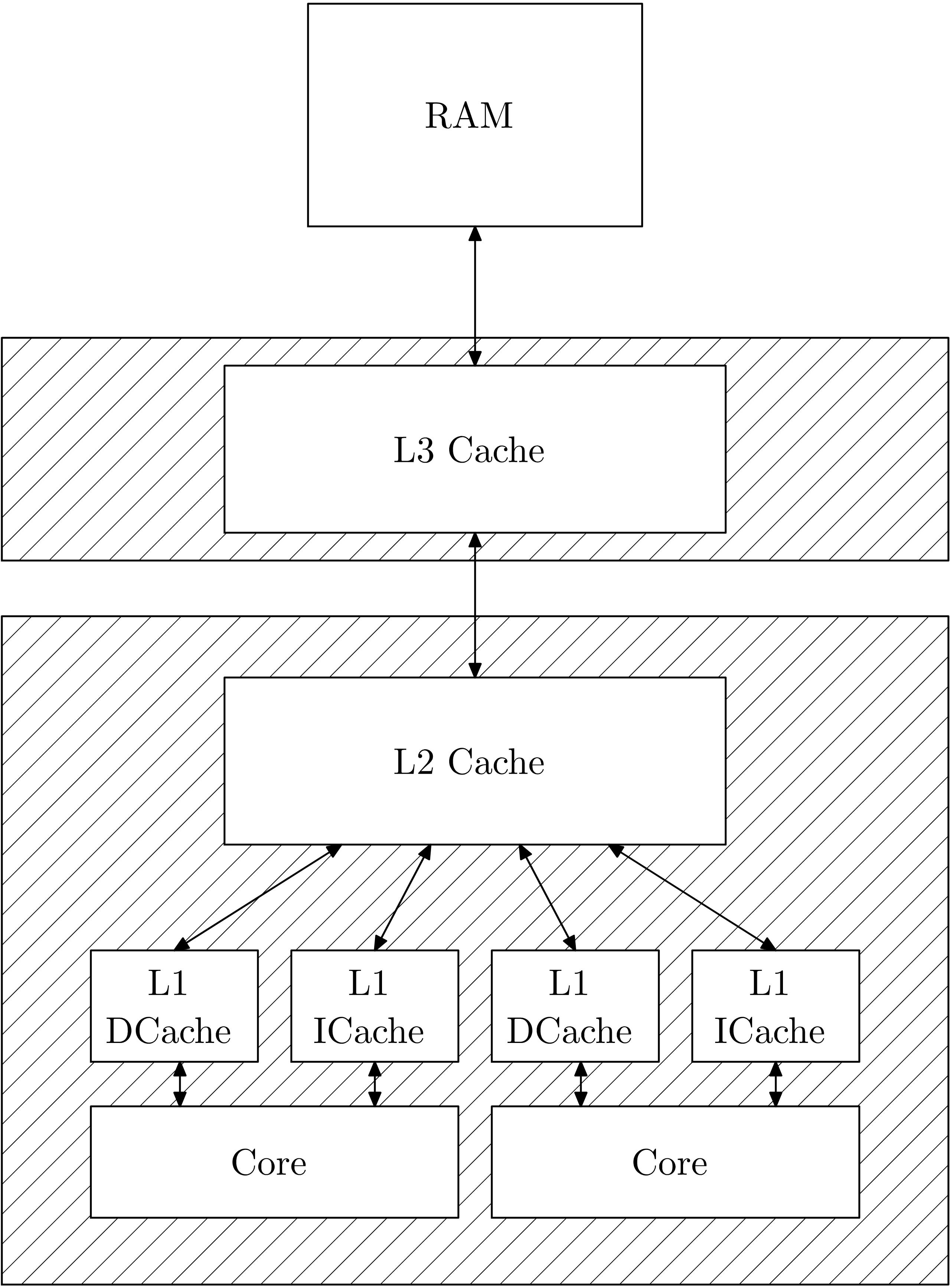
Diagram inspired by Ferruccio Zulian.
The L1 cache has the fastest memory access, followed by L2, L3, and then RAM. To exploit the L1 speed, we use a technique known as cache warming, i.e. keeping the resources we need continuously close to the compute cores.
A good illustration to keep in mind is the following infographic:
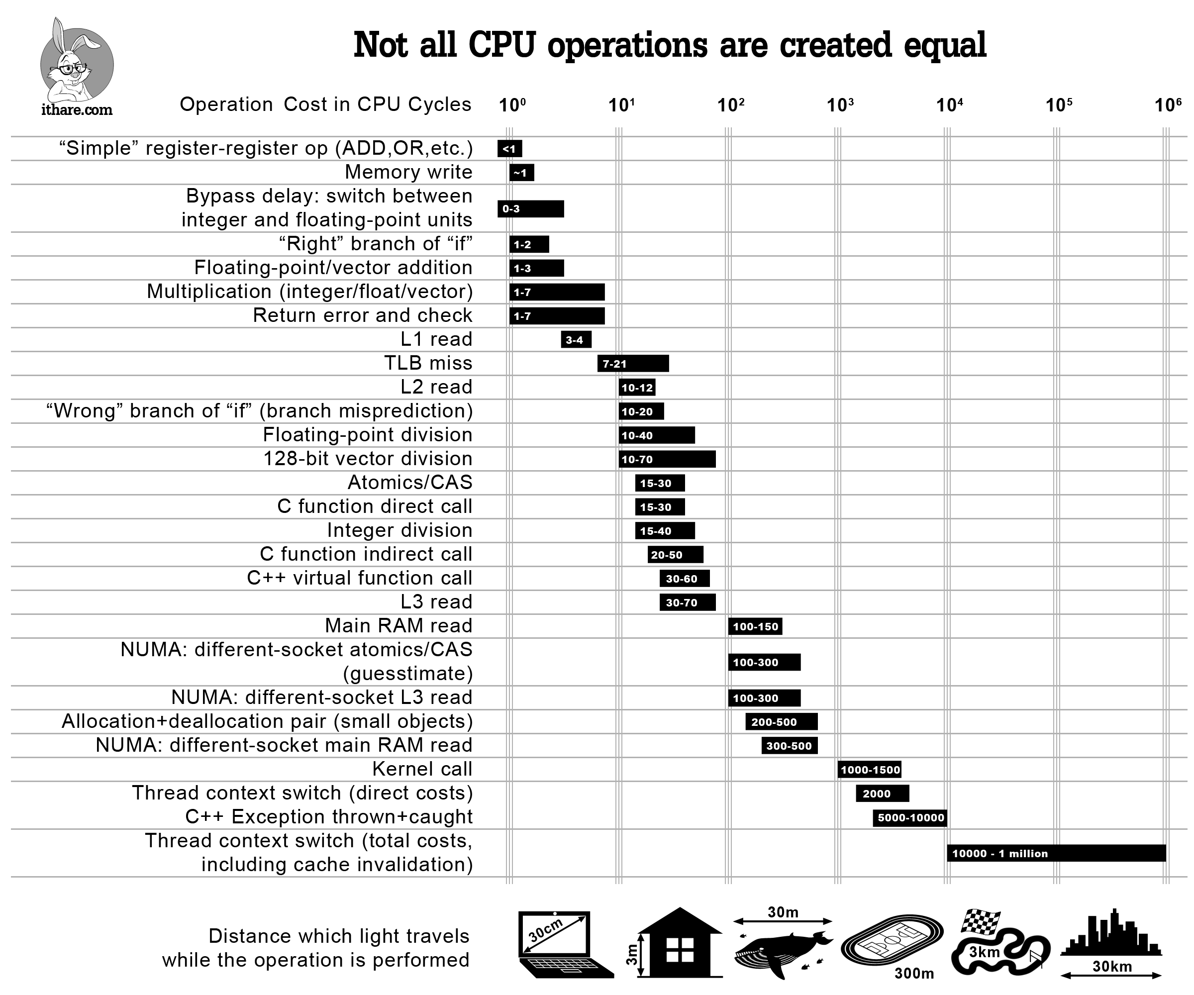
We can illustrate this memory overhead in terms of cache lines and array structures.
Array ordering and cache lines
Modern CPUs try to predict what is needed in the cache; e.g. for arrays, a cache line is loaded into the CPU cache, which is the next chunk of an array.
In the case of one dimensional arrays, this is straight forward to visualise: a cache line may fit $n$ values, thus $n$ contiguous values are loaded into the cache so that iterating over the array is faster.
When the arrays are multi dimensional, different languages abstract how the memory is stored in their interface; the two common systems are row- and column-major memory layouts.
For column major layouts, each column is stored top to bottom in a one dimensional array continuously, whereas in row major layouts, the rows are stored side to side.
To make best use of the cache, we want to ensure we are iterating over the major layout; consider:
using BenchmarkTools

A = rand(500, 500)
B = rand(500, 500)
C = rand(500, 500)

function inner_rows!(C,A,B)
  for i in 1:500, j in 1:500
    C[i,j] = A[i,j] + B[i,j]
  end
end
inner_rows! (generic function with 1 method)
The above iterates over the rows of the two dimensional array, before incrementing the column count.
@benchmark inner_rows!($C, $A, $B)
BenchmarkTools.Trial: 9779 samples with 1 evaluation.
 Range (min … max):  475.324 μs …  1.224 ms  ┊ GC (min … max): 0.00% … 0.00%
 Time  (median):     494.925 μs              ┊ GC (median):    0.00%
 Time  (mean ± σ):   508.100 μs ± 49.391 μs  ┊ GC (mean ± σ):  0.00% ± 0.00%

  ▅▆▆██▆▆▆▅▄▄▂▁  ▁▁▁▁                                          ▂
  ██████████████████████▇▇▇███▇▇█▇█▇▇▆▇▆▆▅▆▅▅▅▅▄▆▅▂▆▄▄▄▄▆▅▅▄▅▅ █
  475 μs        Histogram: log(frequency) by time       730 μs <

 Memory estimate: 0 bytes, allocs estimate: 0.
Performing the same operation, but iterating over the columns first:
function inner_cols!(C,A,B)
  for j in 1:500, i in 1:500
    C[i,j] = A[i,j] + B[i,j]
  end
end
inner_cols! (generic function with 1 method)
Will yield a dramatic performance improvement:
@benchmark inner_cols!($C, $A, $B)
BenchmarkTools.Trial: 10000 samples with 1 evaluation.
 Range (min … max):  303.785 μs … 762.236 μs  ┊ GC (min … max): 0.00% … 0.00%
 Time  (median):     378.531 μs               ┊ GC (median):    0.00%
 Time  (mean ± σ):   380.954 μs ±  42.000 μs  ┊ GC (mean ± σ):  0.00% ± 0.00%

  ▁ ▆▂▅▂▁         ▄▂▇█▅▄▄▃▄▄▄▄▄▃▃▂▂▁▁▁                          ▂
  █▇██████████▆██▇██████████████████████▇█▇▇▇▇▇▅▆▅▆▇▆▆▅▆▆▅▅▆▅▄▆ █
  304 μs        Histogram: log(frequency) by time        536 μs <

 Memory estimate: 0 bytes, allocs estimate: 0.
Note: Julia is column major, whereas Python (numpy) is row major.
Broadcasting
Julia’s broadcast mechanism generates and JIT compiles Julia functions on the fly. Compare this to, e.g. numpy, which has a specifc C API it relies on, and thus cannot adapt well to combinations of operations, as each operation calls a different C function, instead of combining the operations into a single (Julia) function.
Views
Slices in Julia default allocate, unless prefixed with @view or a block with @views.
Summary
Important points:
iterate along layout major
avoid heap allocations (heap allocations happen when size not known at compile time)
mutate to avoid heap allocations
fuse broadcasts; prefer
@.instead of many.+,.=, etc.Julia loops are as fast as C, thus array vectorisation offers little benefit (standard algorithms just help reading intent)
use views instead of slices to avoid (copy) allocations
avoid heap allocations for O(n)
Use a library abstraction like StaticArrays.jl to avoid heap allocations.
Multiple dispatch
Julia uses type inferrence to optimize memory; a function written in Julia without types is known as a generic function:
f(x, y) = x + y
f (generic function with 1 method)
In contrast to other generic functions in other languages, a Julia generic is not a single function, but rather is compiled to inferred types when invoked. This can be demonstrated by examining the LLVM intermediate representation (IR) using a Julia macro:
@code_llvm f(2, 5)
;  @ In[5]:1 within `f'
define i64 @julia_f_1707(i64 signext %0, i64 signext %1) {
top:
; ┌ @ int.jl:87 within `+'
   %2 = add i64 %1, %0
; └
  ret i64 %2
}
Here, the type inferred was i64. By contrast:
@code_llvm f(2.0, 5.0)
;  @ In[5]:1 within `f'
define double @julia_f_1742(double %0, double %1) {
top:
; ┌ @ float.jl:326 within `+'
   %2 = fadd double %0, %1
; └
  ret double %2
}
The inferred type is now double.
A Julia generic is then actually a family of functions, with a new one compiled each time it is called with a new type combination:
@code_llvm f(2, 5.0)
;  @ In[5]:1 within `f'
define double @julia_f_1744(i64 signext %0, double %1) {
top:
; ┌ @ promotion.jl:321 within `+'
; │┌ @ promotion.jl:292 within `promote'
; ││┌ @ promotion.jl:269 within `_promote'
; │││┌ @ number.jl:7 within `convert'
; ││││┌ @ float.jl:94 within `Float64'
       %2 = sitofp i64 %0 to double
; │└└└└
; │ @ promotion.jl:321 within `+' @ float.jl:326
   %3 = fadd double %2, %1
; └
  ret double %3
}
Note that here the return type was inferred as double, and the i64 argument is promoted to a double.
A different Julia macro lets us inspect how the types are being inferred in every operation:
@code_warntype f(2.0, 5)
Variables
  #self#::Core.Const(f)
  x::Float64
  y::Int64

Body::Float64
1 ─ %1 = (x + y)::Float64
└──      return %1
Julia is able to perform this type inferrence as soon as a function is called; consider a more involved example:
function g(x, y)
  a = 4
  b = 2
  c = f(x,a)
  d = f(b,c)
  f(d,y)
end
g (generic function with 1 method)
The types are fully deduced as soon as x and y are inferred:
@code_warntype g(2, 5.0)
Variables
  #self#::Core.Const(g)
  x::Int64
  y::Float64
  d::Int64
  c::Int64
  b::Int64
  a::Int64

Body::Float64
1 ─      (a = 4)
│        (b = 2)
│        (c = Main.f(x, a::Core.Const(4)))
│        (d = Main.f(b::Core.Const(2), c))
│   %5 = Main.f(d, y)::Float64
└──      return %5
And the IR even inlines to optimize further:
@code_llvm g(2, 5.0)
;  @ In[10]:1 within `g'
define double @julia_g_2119(i64 signext %0, double %1) {
top:
;  @ In[10]:5 within `g'
; ┌ @ In[5]:1 within `f'
; │┌ @ int.jl:87 within `+'
    %2 = add i64 %0, 6
; └└
;  @ In[10]:6 within `g'
; ┌ @ In[5]:1 within `f'
; │┌ @ promotion.jl:321 within `+'
; ││┌ @ promotion.jl:292 within `promote'
; │││┌ @ promotion.jl:269 within `_promote'
; ││││┌ @ number.jl:7 within `convert'
; │││││┌ @ float.jl:94 within `Float64'
        %3 = sitofp i64 %2 to double
; ││└└└└
; ││ @ promotion.jl:321 within `+' @ float.jl:326
    %4 = fadd double %3, %1
; └└
  ret double %4
}
Union types
If the types cannot be inferred to a single outcome, Julia will use a type Union to keep the memory as restricted as possible and to be able to compile to the highest degree of optimization:
function h(x, y)
  out = x + y
  rand() < 0.5 ? out : Float64(out)
end
h (generic function with 1 method)
The type deduction here is much more complex, since if x and y are both integers, out will be an integer, and thus the function may either return an Int64 or a Float64:
@code_warntype h(1, 2)
Variables
  #self#::Core.Const(h)
  x::Int64
  y::Int64
  out::Int64

Body::Union{Float64, Int64}
1 ─      (out = x + y)
│   %2 = Main.rand()::Float64
│   %3 = (%2 < 0.5)::Bool
└──      goto #3 if not %3
2 ─      return out
3 ─ %6 = Main.Float64(out)::Float64
└──      return %6
Unions are not quite as optimizeable as single types, however are still allow for much better performance than Any.
Primatives
Julia value types are fully inferrable and composed of primative types, which can be verified with the isbits function:
isbits(1.0)
true
Structs which are entirely value based also are fully inferrable:
struct ComplexNumber_1
    real::Float64
    imag::Float64
end

isbits(ComplexNumber_1(1, 1))
true
Contrast this with a more generically typed:
struct ComplexNumber_2
    real::Number
    imag::Number
end

isbits(ComplexNumber_2(1, 1))
false
Even though
Int64 <: Number
true
We can mitigate this with template generics:
struct ComplexNumber_3{T}
    real::T
    imag::T
end

isbits(ComplexNumber_3(1, 1))
true
Since a different ComplexNumber_3{T} is compiled depending on the arguments, and thus is a concrete type. Such a template generic will optimize well when used any inferrable type.
Finally, note that isbits does not apply to mutable types, since mutable types are heap allocated (unless completely erased by compiler destructuring). Types which are isbits compile down to bit-wise operations in Julia, and thus can be used with other devices, such as GPU kernels.
Function barriers
An array with non-concrete types can lead to un-optimizable code. For example, the array:
x = Number[1.0,3]
2-element Vector{Number}:
 1.0
 3
To fully optimize loops and function calls within a function body, we can use barriers to ensure the dispatched function has stable and concrete types.
Contrast this:
function r(x)
  a = 4
  b = 2
  for i in 1:100
    c = f(x[1],a)
    d = f(b,c)
    a = f(d,x[2])
  end
  a
end

@benchmark r($x)
BenchmarkTools.Trial: 10000 samples with 7 evaluations.
 Range (min … max):  5.178 μs … 191.758 μs  ┊ GC (min … max): 0.00% … 96.53%
 Time  (median):     6.054 μs               ┊ GC (median):    0.00%
 Time  (mean ± σ):   6.268 μs ±   4.518 μs  ┊ GC (mean ± σ):  1.83% ±  2.55%

  ▃▄▁▂▂▁ ▁▅▅█
  ██████▇████▆▃▆▃▄▃▄▃▃▃▆▄▂▂▂▂▂▂▂▂▂▂▂▁▂▂▂▂▂▂▂▂▂▂▂▂▂▂▂▂▂▂▂▂▂▂▂▂ ▃
  5.18 μs         Histogram: frequency by time        11.4 μs <

 Memory estimate: 4.69 KiB, allocs estimate: 300.
With a guarded version:
s(x) = _s(x[1], x[2])

function _s(x1, x2)
  a = 4
  b = 2
  for i in 1:100
    c = f(x1,a)
    d = f(b,c)
    a = f(d,x2)
  end
  a
end

@benchmark s($x)
BenchmarkTools.Trial: 10000 samples with 200 evaluations.
 Range (min … max):  382.470 ns …  1.592 μs  ┊ GC (min … max): 0.00% … 0.00%
 Time  (median):     412.245 ns              ┊ GC (median):    0.00%
 Time  (mean ± σ):   436.922 ns ± 68.642 ns  ┊ GC (mean ± σ):  0.00% ± 0.00%

  ▅  ▇▁█▂▂ ▁ ▁    ▁ ▄▁ ▃  ▂  ▂  ▄▂                             ▁
  █▆▃█████▇█▅█▅█▇▆█▆██▇█▇▅█▆▅█▆▅██▇▅▇▄▅▆▅▄▆▅▅▄▅▅▅▅▃▃▅▄▄▃▅▃▃▃▄▃ █
  382 ns        Histogram: log(frequency) by time       708 ns <

 Memory estimate: 16 bytes, allocs estimate: 1.
The interface of r(x) and s(x) is exactly the same.
The function r(x) cannot type inferr:
@code_warntype r(x)
Variables
  #self#::Core.Const(r)
  x::Vector{Number}
  @_3::Union{Nothing, Tuple{Int64, Int64}}
  b::Int64
  a::Any
  i::Int64
  d::Any
  c::Any

Body::Any
1 ─       (a = 4)
│         (b = 2)
│   %3  = (1:100)::Core.Const(1:100)
│         (@_3 = Base.iterate(%3))
│   %5  = (@_3::Core.Const((1, 1)) === nothing)::Core.Const(false)
│   %6  = Base.not_int(%5)::Core.Const(true)
└──       goto #4 if not %6
2 ┄ %8  = @_3::Tuple{Int64, Int64}::Tuple{Int64, Int64}
│         (i = Core.getfield(%8, 1))
│   %10 = Core.getfield(%8, 2)::Int64
│   %11 = Base.getindex(x, 1)::Number
│         (c = Main.f(%11, a))
│         (d = Main.f(b::Core.Const(2), c))
│   %14 = d::Any
│   %15 = Base.getindex(x, 2)::Number
│         (a = Main.f(%14, %15))
│         (@_3 = Base.iterate(%3, %10))
│   %18 = (@_3 === nothing)::Bool
│   %19 = Base.not_int(%18)::Bool
└──       goto #4 if not %19
3 ─       goto #2
4 ┄       return a
And nor can s(x):
@code_warntype s(x)
Variables
  #self#::Core.Const(s)
  x::Vector{Number}

Body::Any
1 ─ %1 = Base.getindex(x, 1)::Number
│   %2 = Base.getindex(x, 2)::Number
│   %3 = Main._s(%1, %2)::Any
└──      return %3
However, _s may be specialised since %1 and %2 in the IR will be concrete, and the cost is only a single dynamic dispatch.
Summary
Julia is able to optimize well through type inferrence (when concrete types can be inferred)
multiple dispatch leverage type specialisation for minimal- or zero-overhead runtime
ensuring known types in function bodies and loops can drastically improve performance